Equipment
Measuring Lens Variance
Warning: This is a Geek Level 3 article. If you aren’t into that kind of thing, go take some pictures.
I’ve been writing and discussing the copy-to-copy variation that inevitably occurs in lenses since 2008. (1,2,3,4) Many people don’t want to hear about it. Manufacturers don’t want to acknowledge some of their lenses aren’t quite as good as others. Reviewers don’t want to acknowledge that the copy they reviewed may be a little better or a little worse than most copies. Retailers don’t want people exchanging one copy after another trying to find the Holy Grail copy of a given lens. And honestly, most photographers and videographers don’t want to be bothered. They realize lens’ sample variation can make a pretty big difference in the numbers a lens tester or reviewer generates without making much difference in a photograph.
It does matter occasionally, though. I answered an email the other day from someone who said, in frustration, that they had tried 3 copies of a given lens and all were slightly tilted. I responded that I’d lab-tested over 60 copies of that lens, and all were slightly tilted. It wasn’t what he wanted to hear, but it probably saved him some and his retailer some frustration. There’s another lens that comes in two flavors: very sharp in the center but weaker in the corners, or not quite as sharp in the center but stronger in the corners. We’ve adjusted dozens of them and can give you one or the other. Not to mention sample variation is one of the causes that make one review of a lens say it’s poor, when other reviewers found it to be great.
At any rate, copy variation is something few people investigate. And by few, I mean basically nobody. It takes a lot of copies of a lens and some really good testing equipment to look into the issue. We have lots of copies of lenses and really good testing equipment, and I’ve wanted to quantify sample variation for several years. But it’s really, really time-consuming.
Our summer intern, Brandon Dube, has tackled that problem and come up with a reasonably elegant solution. He’s written some Matlab scripts that grab the results generated from our Trioptics Imagemaster Optical Bench, summarizes them, and performs sample variation comparisons automatically. We’re going to eventually present that data to you just like we present MTF data: when a new lens is released we’ll also give you an idea of the expected sample variation. Before we do that though, we need to get some idea of what kind of sample variations should be expected.
For today, I’m going to mostly introduce the methods we’re using. Why? Because I’m old fashioned enough to think scientific methods are still valid. If I claim this lens scores 3.75 and that lens scores 5.21, you deserve to know EXACTLY what those findings mean (or don’t mean) and what methods I used to reach those findings. You should, if you want to, be able to go get your own lenses and testing equipment and duplicate those findings. And maybe you can give us some input that helps us refine our methods. That’s how science works.
I could just pat you on the head, blow some smoke up your backside, call my methods proprietary and too complex, and tell you this lens scores 3.75 and that lens scores 5.21, so you should run out and buy that. That provides hours of enjoyment fueling fanboy duels on various forums, but otherwise is patronizing and meaningless. Numbers given that way are as valid as the number of the Holy Hand Grenade of Antioch.
Methods
All lenses were prescreened using our standard optical testing to make certain the copies tested were not grossly decentered or tilted. Lenses were then measured at 10, 20 ,30, 40, and 50 line pairs per mm using our Trioptics Imagemaster MTF bench. Measurements were taken at 20 points from one edge to the other and repeated at 4 different rotations (0, 45, 90, and 135 degrees), giving us a complete picture of the lens.
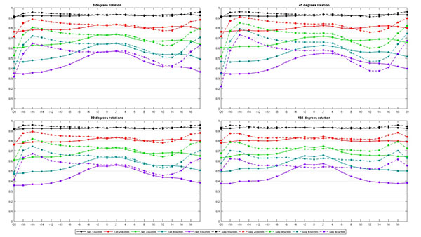
The 4 rotation values were then averaged for each copy, giving as a graph like this for each copy.
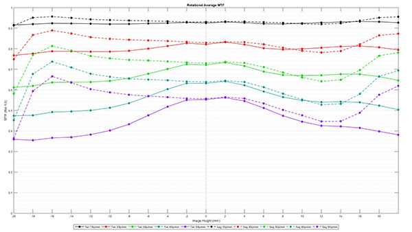
The averages for 10 copies of the same lens model were then averaged, giving us an average MTF curve for the 10 copies of that lens. This is the type of MTF reading we show you in a blog post. The graphics are a bit different than we’ve been using, but that’s because we’re generating these with one of Brandon’s scripts now, so they’ll be more reproducible now.
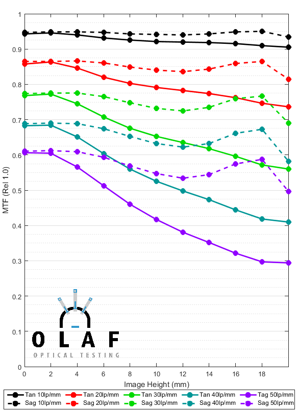
- Graph 1: Average MTF of 10 copies of a lens.
Graphing the Variation Between Copies
Every copy of the lens is slightly different than this ‘average’ MTF and we want to give you some idea of how much variance exists between copies. A simple way is to calculate the standard deviation at each image height. Below is a graph showing the average value as lines, with the shaded area representing 1.5 standard deviations above and below the average. In theory, (the theory doesn’t completely apply here, but it gives us a reasonable rule of thumb) MTF results for 98% of all copies of this lens would fall within the shaded areas.
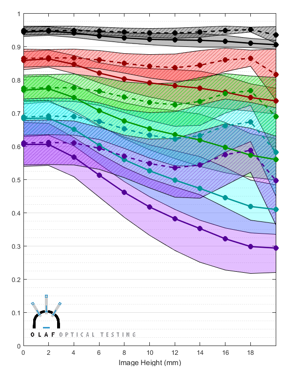
- Graph 2: Average MTF (lines) +/- 1.5 S. D. (area)
Obviously, these area graphs overlap so much that it’s difficult to tell where the areas start and stop. We could change to 1 or even 0.5 standard deviations and make things look better. That would work fine for the lens we used in this example, but this is actually a lens with fairly low variation. Some other lenses vary so much that they would just make a graph that basically is nothing but completely overlapping colors, even if we showed +/- one standard deviation.
The problem of displaying lens variation is one we’ve struggled with for years; most variation for most lenses just won’t fit in the standard MTF scale. We have chosen to scale the variance chart by adding 1.0 to the 10lp/mm value, 0.9 to the 20 lp/mm value, 0.75 to 30lp/mm, 0.4 to 40lp/mm, and 0.15 to 50lp/mm. We chose those numbers simply because they make the graphs readable for a “typical” lens.
Graph 3 presents the same information as Graph 2 above, but with the axis expanded as we described to make the variation more readable.
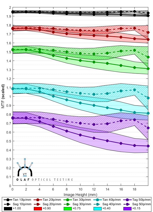
- Graph 3: Average MTF (lines) +/- 1.5 S. D. (area); modified vertical axis
You could do some math in your head and still get the MTF numbers off of the new graph, but we will, of course, still present average MTF data in the normal way. This graph will only be used to illustrate variance. It can be quite useful, though. For example, the figure below compares the graph for the lens we’ve been looking at on the left, and a different lens on the right.

Some things are very obvious at a glance. The second lens clearly has lower MTF than the first lens. It also has a larger variation between samples, especially as you go further away from the center (center is the left side of the horizontal axis). In the outer 1/3 of the lens, in particular, the variation is extremely large. This agrees with what we see in real life: the second lens is one of those lenses that every copy seems to have at least one bad corner, and some more than one bad corner. Also if you look at the black and red areas at the center of each lens (the left side of each graph) even the center of the second lens has a lot of variation between copies. Those are the 10 and 20 line pairs per mm graphs and these differences between copies in the center are the kind of thing that most photographers would notice as a ‘soft’ or ‘sharp’ copy.
The Variation Number
The graphs are very useful to compare two or three different lenses, but we intend to compare variation for a lot of different lenses. With that in mind we thought a numeric ‘variation number’ would be a nice thing to generate. A table of numbers certainly provides a nice, quick summary that would be useful for comparing dozens of different lenses.
As a rule, I hate when someone ‘scores’ a lens or camera and tries to sum up 674 different subjective things by saying ‘this one rates 6.4353 and this one rates 7.1263’. I double-secret hate it when they use ‘special proprietary formulas you wouldn’t understand’ to generate that number. But this number is only describing one thing: copy-to-copy variation. So I think if we show you exactly how we generate the number then 98% of you will understand it and take it for what it is, a quick summary. It’s not going to replace the graphs, but may help you decide which graphs you want to look at more carefully.
(<Geek on>)
It’s a fairly straightforward process to find the number of standard deviations needed to satisfy some absolute limits, for example, +/-12.5%. Just using the absolute standard deviation number though, would penalize lenses with high MTF. If the absolute MTF is 0.1, there’s not much room to go up or down while if it’s 0.6, there’s lots of room to change. This meant bad lenses would seem to have low variation scores while good lenses would have higher scores. So we made the Variation number relative to the lens’ measured MTF, rather than an absolute variation. We simulated the score for lenses of increasingly high resolution and saw the score would rise exponentially, so we take the square root of it to make it close to linear.
Initially we thought we’d just find the worst area of variability for each lens, but we realized some lenses have low variation across most of the image plane and then vary dramatically in the last mm or two. Using the worst location made these lenses seem worse than lenses that varied a fair amount in the center. So we decided to average the lens’ MTF across the entire image plane. To keep the math reasonable, we calculated the number just for the 30 line pair per mm (green area in the graphs) variance, since that is closest to the Nyquist frequency of 24MP-class full-frame sensors. Not to mention, higher frequencies tend to have massive variation in many lenses, while lower frequencies have less variation; 30lp/mm provides a good balance. Since some lenses have more variation in the tangential plane and others the sagittal, we pick the worse of the two image planes to generate the variance number.
Finally we scale the score to get a reasonable scale.
For those who speak computer better than we can explain the formula in words, here’s the exact Matlab code we use:
T3Mean = mean(MultiCopyTan30);
S3Mean = mean(MultiCopySag30);
Tan30SD_Average = mean(MultiCopySDTan30);
Sag30SD_Average = mean(MultiCopySDSag30);
ScoreScale = 9;
if T3Mean > S3Mean
 TarNum = 0.125*T3Mean;
else
 TarNum = 0.125*S3Mean;
end
if Tan30SD_Average > Sag30SD_Average
 ScoreTarget = TarNum*T3Mean;
 VarianceScore = ScoreTarget/Tan30SD_Average;
 MTFAdjustment = 1 - (T3Mean/(0.25*ScoreScale));
 VarianceScore = sqrt(VarianceScore*MTFAdjustment);
else
 ScoreTarget = TarNum*S3Mean;
 VarianceScore = ScoreTarget/Sag30SD_Average;
 MTFAdjustment = 1 - (S3Mean/(0.25*ScoreScale));
 VarianceScore = sqrt(VarianceScore*MTFAdjustment);
end
VarianceNumber = VarianceScore*ScoreScale;
(</Geek off)
Here are some basics about the variance number —
- A high score means there is little variation between copies. If a lens has a variance number of over 7, all copies are pretty similar. If it has a number less than 4, there’s a lot of difference between copies. Most lenses are somewhere in between.
- A difference of “0.5” between two lenses seems to agree with our experience testing thousands of lenses. A lens with a variability score of 4 is noticeably more variable than a lens scoring 5, and if we check carefully is a bit more variable than one scoring 4.5
- A difference of about 0.3 is mathematically significant between lenses of similar resolution across the frame.
- Ten copies of each lens is the most we have the resources to do right now. That’s not enough to do rigid statistical analysis, but it does give us a reasonable idea. In testing 10 copies of nearly 50 different lenses so far, the variation number changes very little between 5 and 10 copies and really doesn’t change much at all after 10 copies. Below is an example of how the variance number changes as we did a run of 15 copies of a lens.
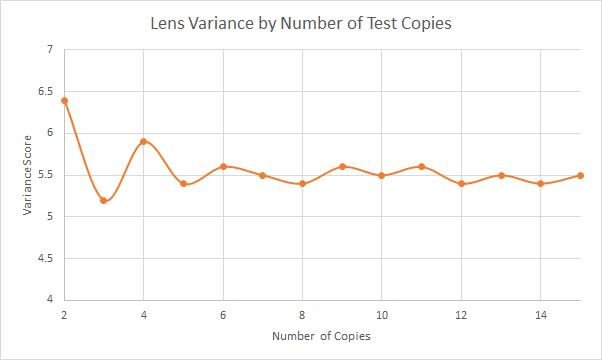
- How the variance number changed as we tested more copies of a given lens. For most lenses, the number was pretty accurate by 5 copies and changed by only 0.1 or so as more copies were added to the average.
Some Example Results
The main purpose of this post is to explain what we’re doing, but I wanted to include an example just to show you what to expect. Here are the results for all of the 24mm f/1.4 lenses you can currently buy for an EF or F mount camera.
First, let’s look at the MTF graphs for these lenses. I won’t make any major comments about the MTF of the various lenses, other than to say the Sigma is slightly the best and the Rokinon much worse than the others.
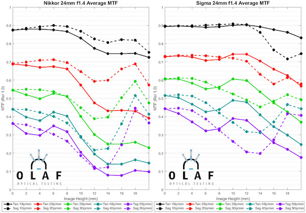
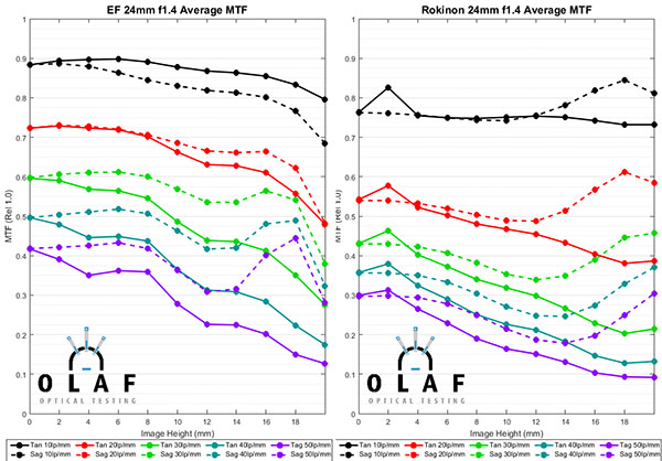
Now lets look at the copy-to-copy variation for the same for lenses. The graphs below also include the Variation Number for each lens, in bold type at the bottom.
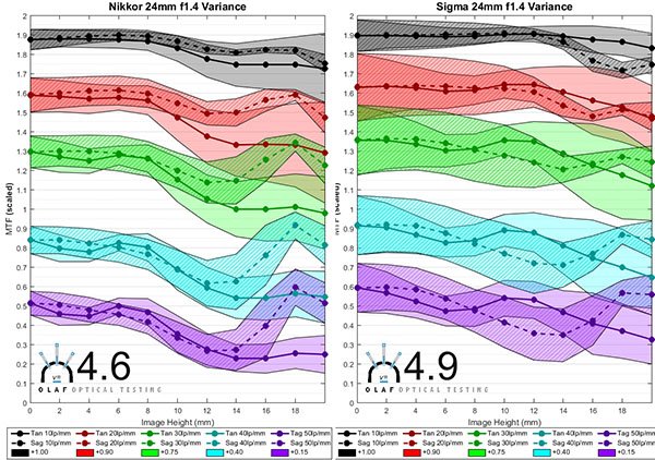
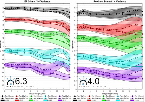
Just looking at the variation number, the Canon 24mm f/1.4L lens has less copy-to-copy variation than the other 24mm f/1.4 lenses. The Rokinon has the most variation.
The Nikon and Sigma lenses show an interesting point. Looking at the graphs the Sigma clearly has more variation, but the Sigma variation number is only slightly different than the Nikon number. That’s because the average resolution of the Sigma is also quite a bit higher at 30lp/mm and the formula we use considers that. If you look at the green variation areas you can see that the weaker Sigma copies will still be as good as the better Nikon copies. But this is a good example of how the number, while simpler to look at, doesn’t give the whole picture.
The graphs show something else that is more important than the simple difference in variation number. The Sigma lens tends to vary much more in the center of the image (left side of the graph) and the variation includes the low frequency 10 and 20 line pairs per mm areas (black and red). The Rokinon tends to vary extremely in the edges and corners (right side of the graph). In the practical world, a photographer carefully comparing several copies of the Sigma would be more likely to notice a slight difference in overall sharpness between the lenses. The same person doing careful testing on several copies of the Rokinon would probably find each lens has a soft corner or two soft corners.
Attention Fanboys: Don’t use this one lens example and start making claims about this brand or that brand. We’ll be showing you in future posts that at other focal lengths things are very different. Canon L lenses don’t always have the least amount of copy-to-copy variation. Sigma Art lenses in other focal lengths do quite a bit better than this. We specifically chose 24mm f/1.4 lenses for this example because they are complicated and are very difficult to assemble consistently.
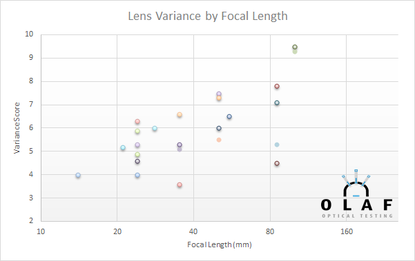
And just for a teaser of things to come, I’ll give you one graph that I think you’ll find interesting, not because it’s surprising, but because it verifies something most of us already know. The graph below is simply a chart of variation number of many lenses, sorted by focal length. The lens names are removed because I’m not going to start fanboy wars without giving more complete information. And that will have to wait a week or two because I’ll be out of town next week. But the graph does show that wider-angle lenses tend to have more copy-to-copy variation (lower variation number), while longer focal lengths, up to 100mm, tend to have less variation. At most focal lengths, though, there are some lenses that have little, and some lenses that have a lot of copy-to-copy variation.
What Are We Going to Do with This?
Fairly soon, we will have this testing done for all wide-angle and standard range prime lenses we carry and can test. (It will be a while before we can test Sony e-mount lenses – we have to make some modifications to our optical bench because of Sony’s electromagnetic focusing.) By the end of August, we expect to have somewhere north of 75 different models tested and scored. It will be useful when you’re considering purchasing a given lens and want to know how different your copy is likely to be than the one you read the review of. But I think there will be some interesting general questions, too.
- Do some brands have more variation than other brands?
- Do more expensive lenses really have less variance than less expensive ones?
- Do lenses designed 20 years ago have more variance than newer lenses? Or do newer, more complex designs have more variance?
- Do lenses with image stabilization have more variance than lenses that don’t?
Before you start guessing in the comments, I should tell you we’ve completed enough testing that I’ve got pretty good ideas of what these answers will be. And no, I’m not going to share until we have all the data collected and tabulated. But we’ll certainly have that done in a couple of weeks.
Roger Cicala, Aaron Closz, and Brandon Dube
Lensrentals.com
June, 2015
A Request:
Please, please don’t send me a thousand emails asking about this lens or that. This project is moving as fast as I can move it. But I have to ‘borrow’ a $200,000 machine for hours to days to test each lens, I have a busy repair department to run, and I’m trying to not write every single weekend. This blog is my hobby, not my livelihood, and I can’t drop everything to test your favorite lens tomorrow.
Author: Roger Cicala
I’m Roger and I am the founder of Lensrentals.com. Hailed as one of the optic nerds here, I enjoy shooting collimated light through 30X microscope objectives in my spare time. When I do take real pictures I like using something different: a Medium format, or Pentax K1, or a Sony RX1R.
-
Randy
-
Charles
-
Leo
-
David Eichler
-
Curby
-
Brandon
-
Wally
-
Brandon
-
Brandon
-
Brandon
-
Wally
-
Matthias Welwarsky
-
JohnL
-
william
-
Florent
-
Feng Chun
-
MayaTlab
-
Fil
-
Carl Spencer
-
Andrew
-
Peter Honka
-
David Ruether
-
Brandon
-
Brandon
-
Brandon
-
Seth
-
Tony
-
JulianH
