Lens Rentals

Throughout the two-century history of photography, the subject of exposure has been repeatedly addressed and hotly debated. In the film era, people talked about exposure and B&W’s negative development in two ways. At first, when most of the photography was done with sheets and plates, it was “expose for the shadows, develop for the highlights”, which assumed a lot of expertise on the part of the practitioner. Then came roll film and standardized development, culminating in the ASA (now ISO) standards for film speed. That existed in parallel with Ansel Adams’ Zone System and other quantitative formulations of the hoary old “expose for the shadows, develop for the highlights”.

Now we’ve got digital cameras, but vestiges of the film era remain. There are light meters in the cameras. There is even a control labeled “ISO” that purports to function like the ASA/ISO rating for film. There are good arguments to be made for why this approach, though having the advantage of familiarity, is sowing confusion, and holding us back in our quest for better photographs.

Cameras, Janus-like, produce both raw files and JPEG ones. Exposing the JPEG files has a fair amount in common with traditional slide film photography, albeit with better dynamic range. However, the ways to get the best exposures for raw files share little with film. The optimal exposure for raw files is rarely the best exposure for JPEG files. This article is about getting the best exposure for raw files, not about how to expose for straight out-of-camera JPEG files. I’ve tried to pitch the text at a middle level. It’s not for beginners, but neither is it one of the dense, experiment-driven, quantitative posts that often populate my blog. I’ll try to keep the math and graphs to a minimum and locate some of them at the end of the article.

What’s the Definition of Exposure?

Wikipedia gets it right:

“In photography, exposure is the amount oflight per unit area (the image plane‘s illuminance times the exposure time) reaching a frame of photographic film or the surface of an electronic image sensor, as determined by shutter speed, lens F-number, and scene luminance.”

The common scientific units for photographic exposure are lux-seconds.

It is common, though somewhat unfortunate, for photographers to ignore the scene luminance, as in this hypothetical exchange:

Q: “What exposure did you use for this image?”
A: “I gave it f/8 at 1/125 second.”

In this article, I’ll try to be explicit when I’m using the more colloquial definition of exposure.

There is yet another photographic definition for exposure: a captured image.

Q: “How many exposures did you make at the wedding?”
A: “More than a thousand. It was spray and pray time.”

In context, this usage is unlikely to be confused with the way I’m using the term in this article.

How Does Exposure Affect Image Noise?

There are several kinds of noise in a digital camera image:

Photon, or shot noise
Read noise, both pre and post-programmable gain.
Processing artifacts
Black point shifts
Quantization noise
Amp glow
Photon response nonuniformity (PRNU)

Don’t worry if you don’t know what some of those are. The long pole in the tent here is photon noise, so you don’t have to worry much about the others. I’m about to explain photon noise, starting with an analogy.

Photons are like raindrops

Richard Feynman used this analogy in a lecture I recently watched on YouTube, and if it’s good enough for him, it’s good enough for me. I was a physics major at Stanford before I switched to electrical engineering, so I knew a fair amount of what Feynman was saying in this lecture. He was presenting to a general audience, and he took great pains to avoid math. I’m sure that helped him communicate with much of his audience, but several times I became confused because he didn’t tell me the math or discuss the matter quantitatively, but instead made hand-wavy, qualitative arguments. To avoid that here, I’m going to give you some information by the qualitative raindrop analogy that follows, and I’m also going to give it to you straight after that. If the straight presentation confuses you, see if the raindrop analogy gets you close to the level of understanding you desire.

Imagine that we want to measure rainfall over an area. We set up square buckets in an array or grid so that they cover the whole area. The buckets are all the same size and the same depth, and they have covers that we can remove or not. The rain starts. The raindrops fall in random locations. Let’s make one unrealistic simplifying assumption: all the raindrops are the same size. We empty all the buckets and remove the covers, thus beginning the exposure of the buckets to the rain. After it’s been raining for a while, we cover the buckets (ending the “exposure”) and measure the depth of the water in each. We map the measurements to a grid on a computer screen, producing an image that represents the amount of rainfall in each bucket.

The faster the rain is falling, the more water, on average, we’ll get in each bucket if the exposure duration is fixed. If it’s raining twice as fast, we can get, on average, the same amount of water by halving the exposure duration. If it’s raining half as fast, we can get, on average, the same amount of water by doubling the exposure duration.

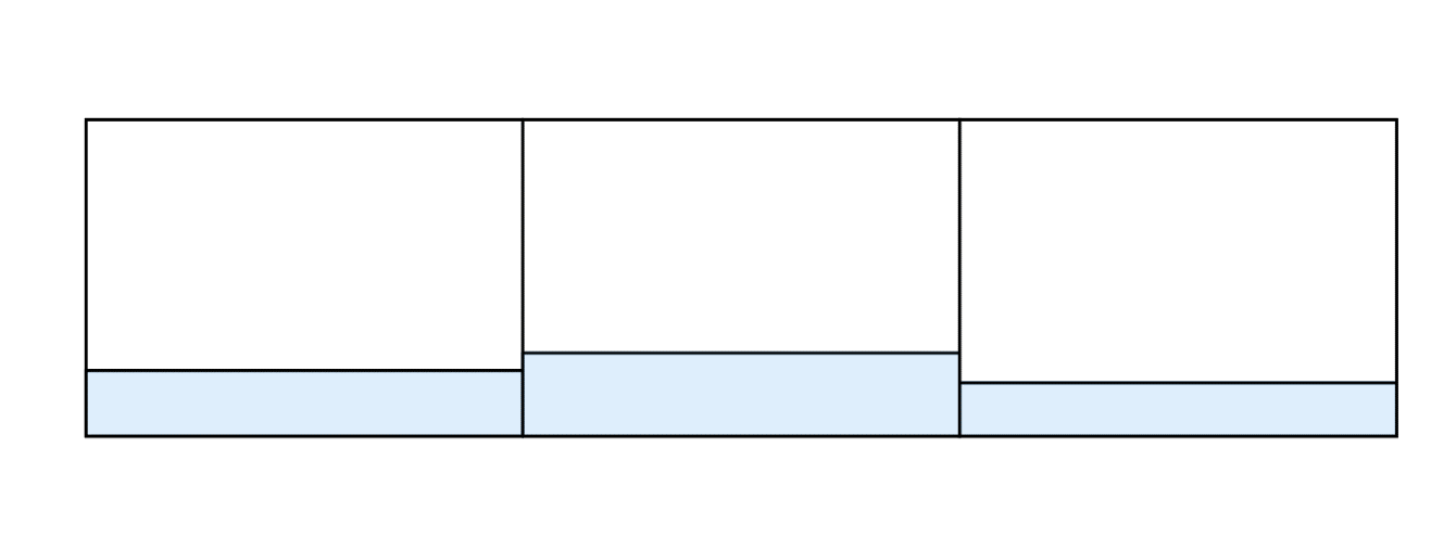
When the rainfall is heavy or the exposure is long, the buckets will be more nearly full at the end of the exposure. If we measure the depth of the water in all the buckets, we’ll notice that there is some variation because of the random nature of the rainfall. If we make several different exposures of varying lengths with the same rain rate, we’ll notice that the longest exposures produce the most variation. We can call that variation “drop noise”. However, if we divide the deviations in each bucket’s measurement from the average by the average measurement for all the buckets, we will find that quantity – call it rainfall signal to drop noise ratio – gets larger the longer the exposure or the faster the rainfall.

Now for what’s actually happening.

Photon noise in the camera

A digital camera sensor converts light to electrons. Like the raindrop measuring, that is inherently noisy. If you make repeated measurements with the same amount of light falling on one pixel, or shine uniform light on a sensor containing many identical pixels, you will get different numbers of electrons for each sample. The histogram of the readings will follow what mathematicians call a Poisson distribution. A property of a Poisson distribution is that the standard deviation in electrons is the square root of the average number of electrons. This is inherent in the process of measuring light intensity, and no amount of clever camera engineering can change it, although there are ways that its effects can be somewhat ameliorated. The more light, the greater the uncertainty, and, with repeated measurements, the greater the noise. The standard deviation of the electrons is also the root mean square (RMS) measure of the noise. Reducing the above to an equation:

Modern CMOS digital cameras are now sufficiently evolved that, in almost all circumstances, the dominant contributor to image noise is photon noise. If you turn the ISO dial up to the nosebleed settings, you may find that read noise of varying descriptions visibly affects the shadows, but I consider most of those images greatly compromised anyway. We’ll get to read noise in due time, but for now, know that photon noise is most likely all you have to worry about.

We saw above that more light means more photon noise. But the scalar metric that best quantifies the visual effect of noise is not the amplitude of the noise itself, but rather the signal-to-noise ratio (SNR), which is the average signal (light, in this case) level divided by the root mean square noise. We want that number to be big. The SNR of photon noise is the average number of electrons divided by the square root of the average number of electrons. If you simplify that fraction, the SNR is the square root of the average number of electrons. That means that the more photons that hit the sensor, the lower the visible noise. In the form of an equation:

Then why not always use the maximum exposure that is possible?

In the raindrop analogy, we don’t want exposures that cause the buckets to overflow, because then we wouldn’t know how much rain fell into that bucket. There is something similar in your digital camera. There are capacitors associated with the photodiodes in the camera sensor. Light knocks electrons loose in the photodiodes, and those electrons charge the capacitors. The more electrons freed by the light hitting the sensor, the more charge on those capacitors. The more charge, the higher the voltage across the capacitors. The voltage is how the camera’s innards determine the number of electrons; it’s a bit like counting pennies by weighing them. At some point, more electrons won’t increase the voltage linearly. This is called saturation, and cameras are usually designed so that the analog to digital converters looking at the voltage on those capacitors reach full scale before the nonlinearity gets too bad.

So, we’ve got two things going on: saturation at the photodiode level, and hard clipping introduced by the analog-to-digital converter. If you put too much light on the sensor, you’re going to get clipping, and thus loss of detail in the brightest parts of the image.

People sometimes talk about clipping of shadow values in raw files. That doesn’t happen. As the amount of light hitting the sensor gets smaller and smaller, the SNR gets worse and worse, until finally the signal is buried in the noise. Hard clipping can affect the bright parts of the image, but the dark areas don’t just suddenly go black (unless there’s something wrong with the black point subtraction).

The parallels between photons and raindrops, and photon noise and drop noise, are:

The statistics of the raindrop counting in our rain gauge are similar to the stats of photon counting in a camera. More raindrops and more photons both improve the signal-to-noise ratio.
You can get more raindrops in the same amount of time when it rains harder. You can get more photons in the same amount of time by making the light brighter or widening the f-stop.
If you want more raindrops but the rain keeps falling at the same rate, you can expose the buckets for longer. If you want more photons but can’t open the aperture or make the light brighter, you can use a longer exposure.
Too many raindrops overflow the buckets and mess up your count. Too many photons saturate the sensor counting system and mess up your image.

We’ll return to the raindrops later.

What are the Characteristics of Good Exposure?

Here’s my list:

Acceptably low noise
Realistic detail in all areas important to the photographer
Adequate depth of field
Acceptable diffraction blur
Acceptable lens aberration blur
Acceptable subject motion blur
Acceptable camera motion blur

Exposure is usually a compromise; many of the above trade off against each other. The definition of acceptable, adequate, and realistic depend on the photographer’s intent, the lighting, the subject, the scene, the way the final image will be presented, and probably a few other things that aren’t occurring to me now.

Good exposure is therefore subjective and squishy. Does that mean that we can’t say anything objective about it? Thankfully, it does not.

Let’s take a few things as givens:

The scene lighting.
The desired depth of field and therefore the desired widest f-stop. Let’s assume that that f-stop produces acceptable lens aberration blur and acceptable diffraction blur.
The acceptable subject and camera motion blur, and therefore the longest allowable shutter speed.

Because of photon noise, we want as much light as we can get on the sensor subject to the above constraints. But there’s an additional constraint: we don’t want any important highlight to be clipped in any raw channel (if I may return to the rainfall and the buckets, we don’t want any of the buckets overflowing). Modern raw converters like Adobe Camera Raw and Lightroom can make guesses if only one or two raw channels are clipped, but that’s for saving a botched capture, not something to plan for.

Raw exposure is like the game of Blackjack. In Blackjack, you want the highest score possible as long as it’s 21 or less, and if your score is more than 21, you lose. In exposure, you want the most light possible as long as significant highlights are not clipped. Like Blackjack, you can win if your exposure produces electron counts a bit under your target, but you lose if it goes over your target. As in Blackjack, if you get greedy, you are likely to pay a price for your greed.

ISO

I’ve spent a lot of time talking about exposure, and so far, I haven’t mentioned ISO settings. That’s not an accident. ISO settings aren’t part of exposure, and ISO settings don’t determine exposure for the thinking photographer. And the ISO setting you choose, also like in Blackjack, can be less than optimum and you’ll be fine, but if it’s higher than optimum, you – or your image — can go bust.

To get an idea of how ISO works, let’s go back to the rainfall and the buckets, but we’ll make a change that Richard Feynman didn’t contemplate. Instead of square open buckets, imagine square funnels of the same size as the buckets were. Below the funnels, we can put buckets of various sizes that are all the same height as the original buckets. If we put the original buckets under the funnels, we’ve got what I’ll call the “base ISO” situation, and everything works as it did before. But now let’s put buckets that are smaller looking down from the top, but the same height. If we put buckets down that is half the area, the same amount of rainfall that got the base ISO buckets half full will fill the smaller buckets (call them the one stop up from base ISO buckets) all the way up.

Why would we have buckets of different sizes? Let’s say that we can only read our measuring scale to 1/16^th of an inch. We’d have half the uncertainly as to how much rain had fallen in each bucket with the half-area buckets, with the downside that if we let the exposure go on too long or it rained too hard, the half-area bucket would overflow, and then we wouldn’t even have an approximate idea of how much rain we’d gotten, though we would have a lower bound. There’s another possible source of uncertainty. Let’s say the water isn’t quite still when we measure it, so there’s a bit of noise that affects what we measure. Let’s call the first one quantization error, and the second one, read noise.

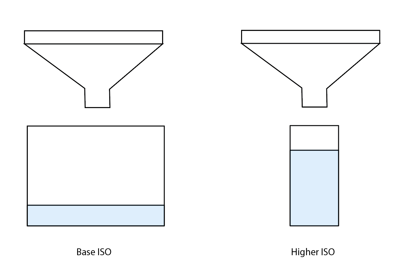
The ISO setting on a digital camera can affect the image in various ways, so the raindrop analogy sometimes isn’t completely apt, but in general, the above should give you a feel for the good and the bad effects of increasing the ISO setting (making the buckets smaller in area). The win is that you can get somewhat more accurate readings. The loss is that there is a greater potential for clipping highlights.

With modern cameras having 14-bit precision or more, the quantizing error is not a limiting factor at any ISO setting and exposure, and increasing ISO doesn’t buy us any reduction in quantizing uncertainty. There is some reduction in read noise as ISO goes up, but in dual conversion gain cameras, the benefits virtually cease soon after the camera switches to high conversion gain mode. I’ll demonstrate those things with a technical discussion in part two of this topic, published in a few days.

And that concludes part one of this two-part article. Hopefully, this gave you a basic understanding of how exposure works, and how photon noise affects the proper raw exposure. In the second half of this article (to be published next week), we’ll go over how to put this knowledge into practice, to get the best exposure possible for your images.

Geek Articles

How to Expose Raw Files – Part 1

What’s the Definition of Exposure?

How Does Exposure Affect Image Noise?

ISO

Related Reading

Author: Jim Kasson

Recent Posts