How to Expose Raw Files – Part 2

This is Part 2 of an article published last week. For the best understanding, please read part one by clicking here.

Last week, we talked a bit about how the camera exposes raw files and used an analogy of rainwater and buckets to explain that. Today, we’re going to dive into the topic more and discuss it with more practical techniques and understanding.

Putting this into Practice

The net of all this is that you want to set your camera to base ISO and get as much light on the sensor as you can without saturating it in areas where you want detail. How successful you are at doing that will depend on how bright the lighting is, how far you must stop down to get the depth of field you desire, and how fast a shutter speed you need to deal with camera and subject motion. But there’s an essential problem: how do you know when you’re saturating the camera sensor or clipping the highlights? 

The news on that front is bad. None of your camera metering functions can reliably detect sensor saturation. If you have a mirrorless interchangeable lens camera (MILC), your two best tools are the highlight zebras and the histogram, but even they are flawed. Both the histogram and the zebras have the right idea. If you want to detect clipping set the zebra threshold just below the clipping level and adjust your exposure – remember, we are at base ISO now — so that no meaningful highlights have the zebra warning. Or look at the right side of the histogram and adjust the exposure until the histogram contains data close to the right edge, but there’s no little spike at the right edge that would indicate that some of the image is clipped. The zebras have an advantage over the histogram in that they indicate where in the image the clipping occurs, and I find them easier to see in the finder.

Both the zebras and the histogram suffer from the same basic problem: they are derived from the preview image that you see in the finder of your MILC, or on the LCD screen when you review photos in your DSLR. The JPEG preview image is of lower resolution than the raw file, so you might miss some small blown-out areas. But that’s not the big problem; the wrong data is being displayed. You want to know when the raw file experiences clipping, and the zebras and histograms tell you when an sRGB or Adobe RGB JPEG image, processed as you’ve defined in your camera menus, is clipping. 

Usually, but by no means always, the JPEG-derived histograms and zebras are conservative – they show clipping before the raw file is actually clipped. How conservative they are depends on the spectrum of the lighting and the white balance you’re using in the camera. Some manufacturers are more conservative than others; if you’re using a Nikon Z7 and you’re judging your exposure from the JPEG histogram (the Z7 doesn’t support zebras except in video mode), you’re likely to have raw files that are quite underexposed compared to what you could get away with if you set your exposure by the raw histogram. 

Similarly, when you get your files into your raw developer, the histogram you see there won’t tell you how close you were to clipping a channel in the raw file. The histogram you see in Lightroom or Adobe Camera Raw is the histogram of the developed image. If you develop an image with all the controls left at their default settings, it’s the histogram of an image developed the way the program creators think most people will like most of the time. 

To know how well you’re doing with your raw exposures, you must use a tool that lets you see the raw data directly. I use two such tools: RawDigger and Fast Raw Viewer. Both will show you raw histograms, but their, ahem, focus is different. Fast Raw Viewer is a culling tool with a raw histogram that makes it very useful for sorting. But you can also use it for quality control, to see if you are getting enough light on the sensor or if you have clipped some high values. RawDigger is a one-trick pony, and its trick is deep and varied analysis of raw files. It requires some learning, but it can yield lots of information. 

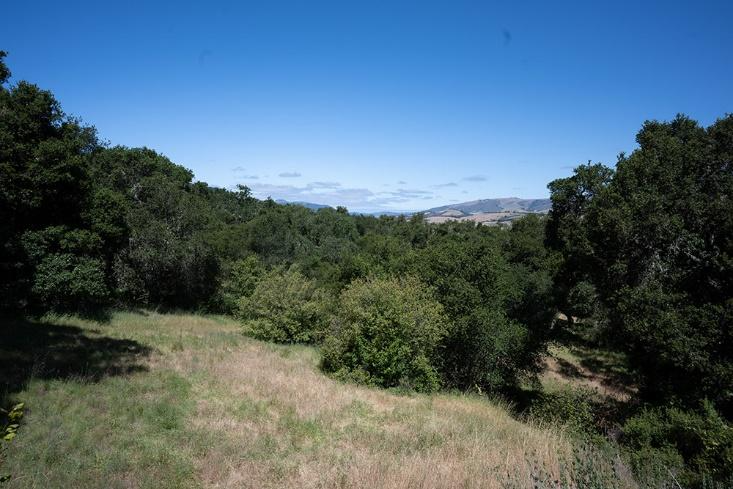
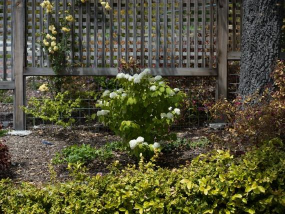
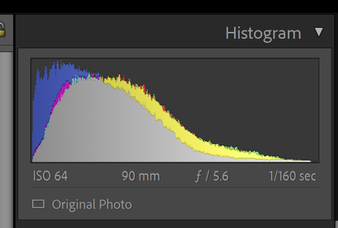
Here’s an example of a raw histogram and the histogram you see in Lightroom. I shot this scene with a Nikon Z7.

Here’s what the histogram in Adobe Camera Raw looks like with the default settings:

Looks like the blue channel is blown, doesn’t it?
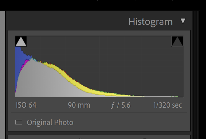
Here’s the Lightroom histogram with default settings:

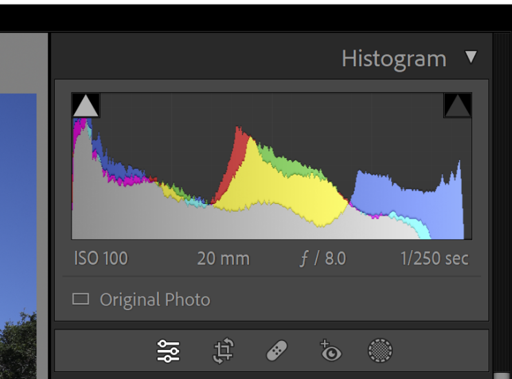
Near the clipping point, it looks similar, as well as it should, since Lightroom and ACR share the same core software; the differences are due to the different color spaces used by the two programs for histograms.

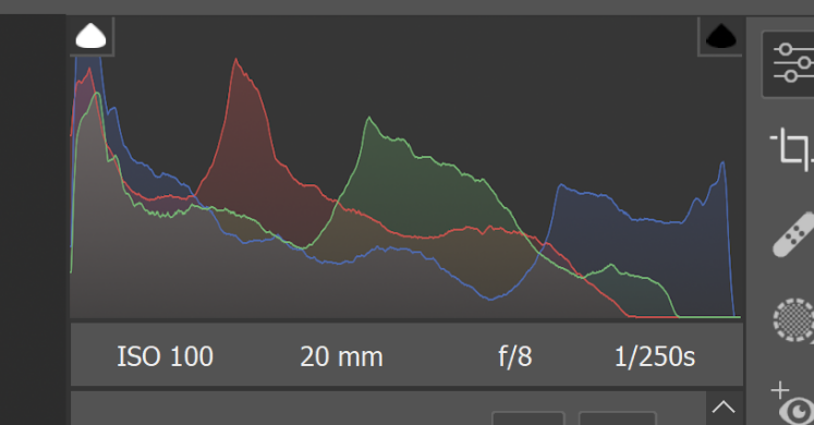
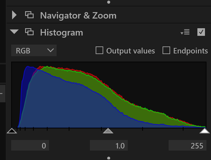
And here’s the raw histogram, courtesy of RawDigger:

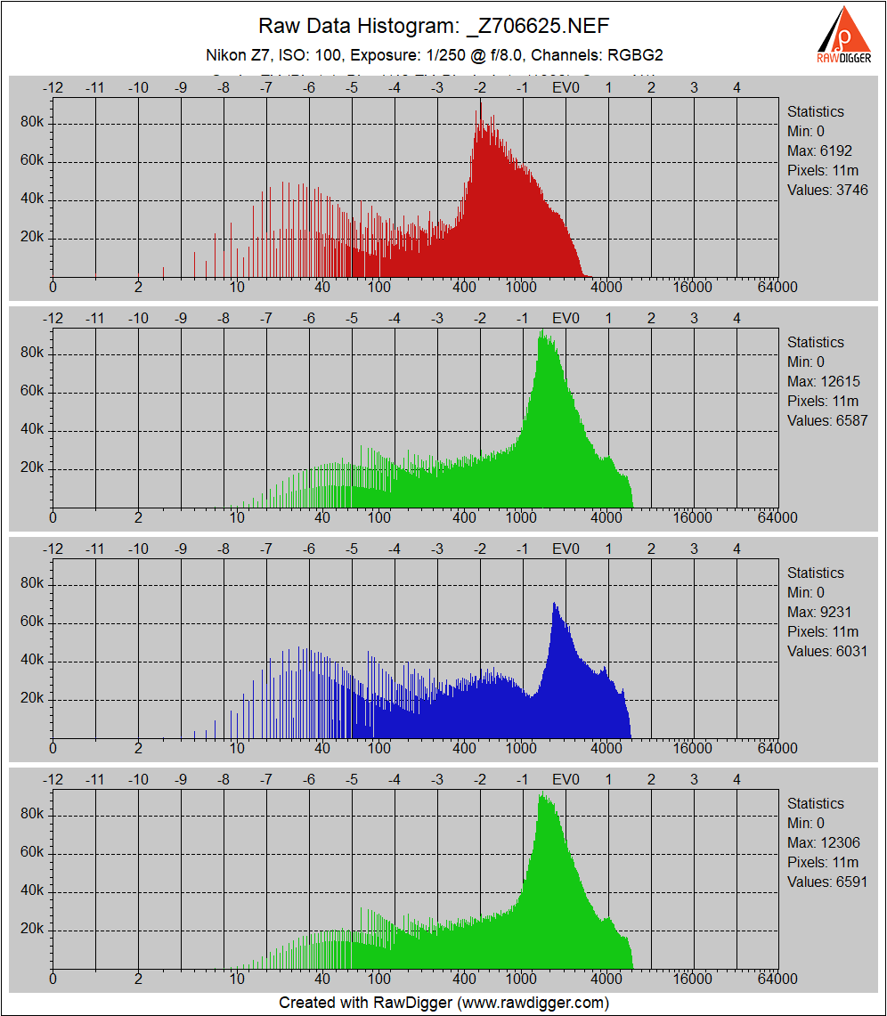
Now we see that the blue raw channel is not the one with the highest values; that honor goes to the green raw channels. And most of the highlights in the blue and green raw channels are about a stop and a half from clipping, which occurs around 16000.

There are things that can be done to make the in-camera histogram more like the raw histogram than it usually is. The most powerful of these is called Uni-WB. These techniques make the finder image look green on most cameras, and, though these approaches have been around for a while, they have not gained much traction in the photographic community. 

How much margin you have depends on the camera and the scene. Here’s an exposed to the right shot with the Hasselblad X2D:

Here’s the raw histogram for that shot:

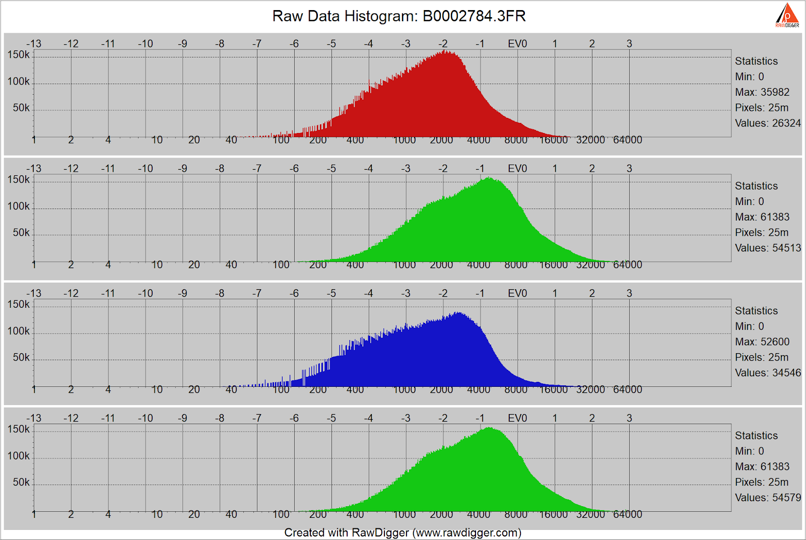
Just a third of a stop more exposure than that shows clipping in the green channels:

This camera saturates at just below 64000; see the spike in the green channels above? 

Here’s the in-camera histogram for the ETTR image:

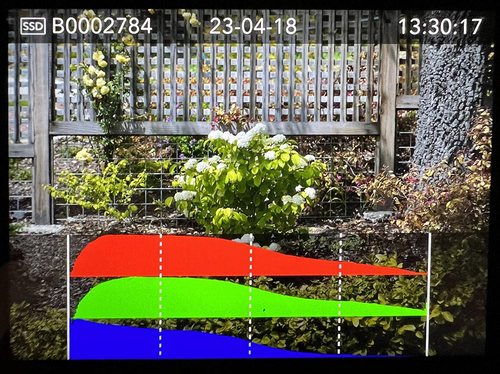
It looks like there is quite a bit of clipping, but the actual raw clipping is minimal. In fact, you must go to an image that is 1 2/3 stops underexposed from the ETTR image to get to the point where the in-camera histogram says there’s no clipping.

If we bring that image into Lightroom with default settings, here’s what we see:

In this case, the Lightroom histogram clipping point isn’t much different from the raw file clipping point. But the shot one stop underexposed from that also shows the histogram going all the way to the right.

Clearly, Lightroom is applying a shoulder to the highlights in the ETTR image.

If we look at the file with Hasselblad’s raw converter, Phocus, here’s the histogram we see with the default settings:

But when we turn the clipping warning on, some of the flowers are tinged in purple:

The take-home lesson is you can’t be sure if the raw file is blown – that’s bad — or just close to it – that’s good – without looking with some program that lets you see the raw data itself.

If you don’t want to look at the raw histograms, you probably won’t have any raw clipping for near-neutral objects lit with common light sources, though you’ll likely be underexposed from true raw ETTR. Be careful around bright colorful objects like flowers, though.

To review, here’s how to get optimum raw exposures:

• Set your ISO to base ISO.
• Set your f-stop to the stop you need to get the depth of field you want.
• Set your shutter speed to get as much or as little blur as you want.
• Check the histogram or the zebras to make sure you’re not going to clip any important highlights.  If you are, stop down or set a faster shutter speed.
• If the histogram shows no information on the right side, consider boosting the ISO setting, but don’t be aggressive about that. If your camera offers dual conversion gain and you want to boost the detail in the deep shadows, you might consider setting the ISO to the lowest setting that gets the high conversion gain. Don’t plan for doing more than a four or five-stop push in postproduction.

Raw Development Implications

If you’re new to this kind of thinking about raw exposure, when you get your images into your favorite raw developer, you may – or may not – be surprised at what you see. 

If you are making images of a typical scene and have not played games with your JPEG preview image controls, your JPEG preview image, its histogram, and the histogram of your raw converter at default settings will reflect a normal-looking capture with histograms that span almost the entire x-axis. Normal processing in your raw developer will work pretty much the way you’d expect it to work. 

If you are shooting a low-contrast scene, you’ll end up with little information on the left side of the in-camera histogram (and the histogram of your raw converter at default settings), and you’ll probably have to darken the midtones and shadow areas in postproduction. But that should work out fine if you’ve gotten enough light on the sensor.

A high-contrast scene with bright highlights that need preserving will probably result in a capture whose JPEG preview image (and the histogram of your raw converter at default settings) is dark, and you’ll need to boost the shadows and midtones in post.

If you’re not interested in some technical details about noise, stop right here, grab your camera, and go make some well-exposed photographs.

Technical Discussion on Quantizing and Read Noise

I know that some of you won’t be satisfied by the raindrop analogy and associated hand-waving. Let’s look quantitatively at how much of a win the good part of increasing ISO buys us. This section assumes some technical knowledge.

First, we’ll look at quantization.  I’ll give numbers for a typical modern CMOS sensor: full well capacity (FWC) 40000 electrons (e-), base ISO 100, 14-bit ADC.

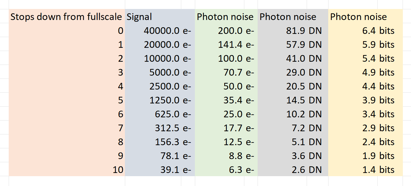
The first column is how far the signal level is below full scale – in stops. The second is the number of electrons in the signal. The third is the root mean square photon noise associated with that electron count. The fourth is the rms value of the photon noise in counts or data numbers. The last column is how many binary digits it would take to capture the rms value of the photon noise. The amount of noise necessary for adequate dither of an analog to digital converter is around 1 bit. Even 10 stops down from full scale the photon noise is dithering the ADC properly. The precision (number of bits) in the ADC is not a limiting factor in the accuracy of the camera. Since we have no read noise in the above analysis, if we looked at more stops down from full scale, we’d eventually get to the point where the photon noise does not provide adequate dither for the ADC.

I’ll look at read noise next, using the Fujifilm GFX 100S as an example. This camera uses a Sony backside illuminated CMOS sensor and is representative of modern sensor pixel designs. Sony, the dominant supplier of sensors for interchangeable lens cameras, uses virtually the same pixel design in sensors for APS-C, full-frame 35mm, 33x44mm medium format, and larger medium format cameras.

Here’s a graph of the input-referred read noise of the GFX 100S versus the ISO setting incremented in 1/3 stop steps, as measured by yours truly with the camera set for 14-bit and 16-bit precision:

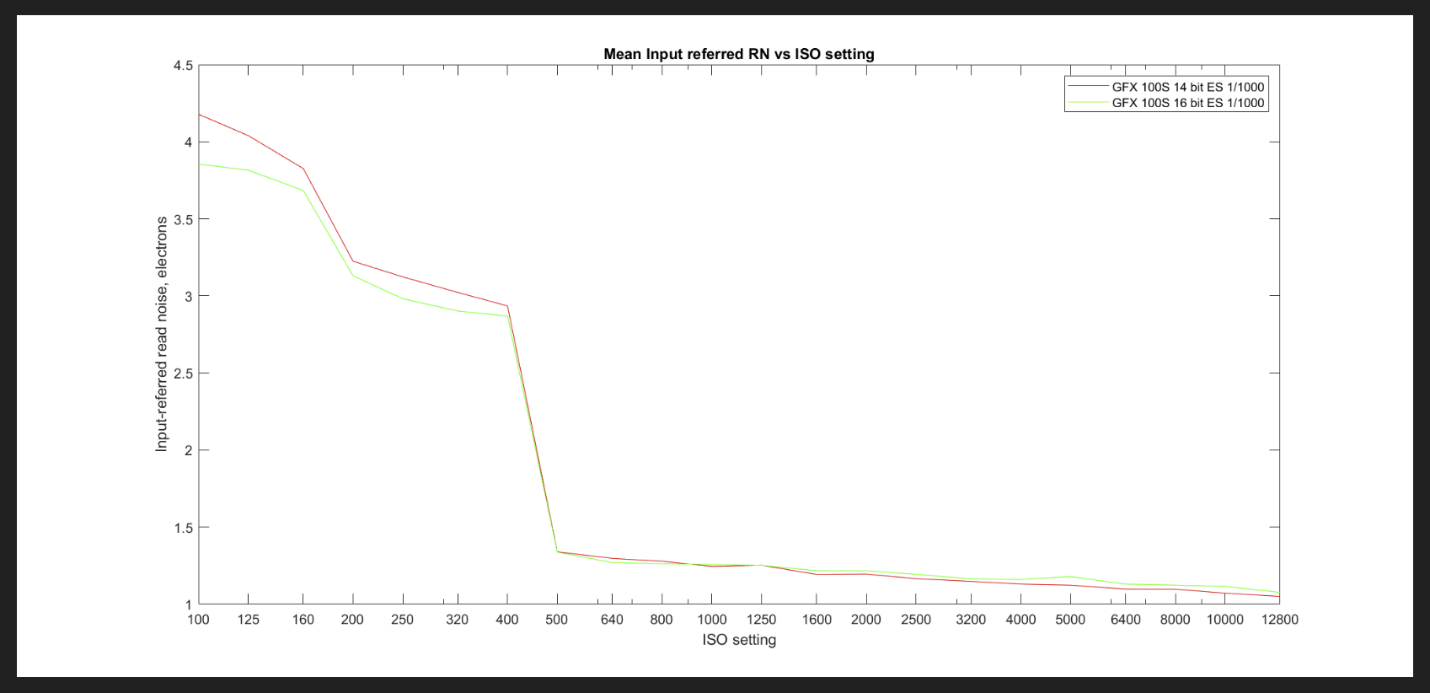
What is input-referred read noise? It is a result of a calculation that uses a black field for the subject and analyzes the noise in the resultant raw file, then calculates how much electron noise on the capacitor in the photodiode there would have to be if that were the only noise in the system. The rain gauge analogy would be calculating the ripple noise in the various-sized buckets in terms of the number of raindrops that would have to fall into the funnel to create that effect. The numbers on the y-axis of this graph are directly comparable to the green column in the photon noise table above.

When you have two uncorrelated noise sources – and photon noise and read noise are uncorrelated – they add as the square root of the sum of the squares. That means that if one source of noise is quite a bit greater than the other, virtually all the noise is coming from that source. Nine stops down from full scale, the photon noise is 8.8 electrons. At ISO 100, the read noise is 4.2 electrons. The total noise is sqrt(8.8^2+4.2^2) or 9.75 electrons.

What if the image is completely dark? Then there’s no photon noise at all. The ISO 100 read noise is 4.4 electrons, that’s almost 2 least significant bits, which is plenty for dithering the ADC. The other place to look at on the curve is at ISO 500, where the higher of the two conversion gains the sensor offers kicks in, that the read noise drops to around 1.4 electrons. That’s almost 3 least significant bits, which is more than enough dither.

Glossary

Dual conversion gain. Conversion gain is the ratio of the voltage on the photodiode capacitor to the number of electrons captured. The conversion gain is set by the capacitance, with lower capacitance producing higher gain. High capacitance allows lower photon noise if enough light falls on the sensor and is desirable at base ISO. Lower capacitance allows lower read noise and is desirable at higher ISOs. Dual conversion gain sensors became popular about 10 years ago, and allow the capacitance to change with ISO setting, thus in some sense allowing the best of both worlds. 

Full well capacity.  Full well capacity (FWC) is the charge that can be stored in a sensor pixel before the pixel saturates. It is measured in electrons (e-). Modern CMOS sensors have FWCs of about 3000 electrons per square micrometer. 

Histogram. A graphical representation of the distribution of numerical data. The x-axis contains intervals, sometimes called buckets. The y-axis plots how many items have values in the range of each bucket. In the histograms presented by cameras, what’s plotted is either scene luminance for the whole frame, or each of the JPEG color channels, also for every pixel in the JPEG preview image. Usually, the in-camera histogram x-axis is linear in the tone curve of the JPEG color space the user selected, which means that middle grays are more or less in the middle of the x axis. In camera histograms have linear y axes. The histogram in Photoshop is in the working color space. The histogram in Lightroom is in the Pro Photo RGB color space, except that is uses the sRBG tone curve. Raw file analyzers like RawDigger offer many ways to bin the image values into buckets and display the results. 

Pixel. Short for picture element; the most basic component of an image. In a sensor, the photodiode electronics associated with the resetting, detection, conversion of electrons to voltage, buffering, and the first stage of switching for one picture element are collectively referred to as a pixel. 

Precision. In computer science, the precision of a numerical quantity is a measure of the detail in which the quantity is expressed. The units are usually binary digits, or bits. The analog to digital converters in cameras output an unsigned binary number. The length of that number in bits is the precision of the ADC. Some people refer to precision as bit depth.

Related Reading

• How Your Camera and Image Processor Determine Colors
• How Your Camera’s Focus Bracketing System Works
• A Brief History of Early Lenses: Part 1
• How the Light Placement Alters Your Subjects

Author: Jim Kasson

I’ve been a photographer since high school, and an electrical engineer all of my professional life. The two things came together for a while. From 1989 until the middle of 1995, I worked as an IBM Fellow at the Almaden Research laboratory south of San Jose, CA. For those six years, my principal area of research was color management, color processing for digital photography, and color transformations such as gamut mapping. At other times in my career, I researched speech recognition and speech bandwidth compression and developed data acquisition and process control computer systems, telephone switching systems, and data communication systems. I retired in 2000, and for the last 22 years when I’m not serving on NFP boards unrelated to photography, I’ve been spending most of my free time making photographs.